Making the Counterfactual Explicit
Suppose a government rolls out a job-training programme in some regions but not others. Administrative earnings records exist for all workers in all regions before and after the rollout. Does an increased average earnings growth in the participating regions prove it worked, or were those regions simply already on faster trajectories? This is a causal question that the administrative record cannot answer on its own.
Whether we’re tracking people, firms or regions, panel data is the record of their repeated measurements over time. The repetition adds leverage and trouble at once. It lets us watch an outcome evolve. It also allows for units to drift onto different trajectories before treatment starts, and it exposes every unit to the same shocks, seasons and anticipation. So the question in this part is not whether outcomes changed. It is what licenses us to call the change causal.
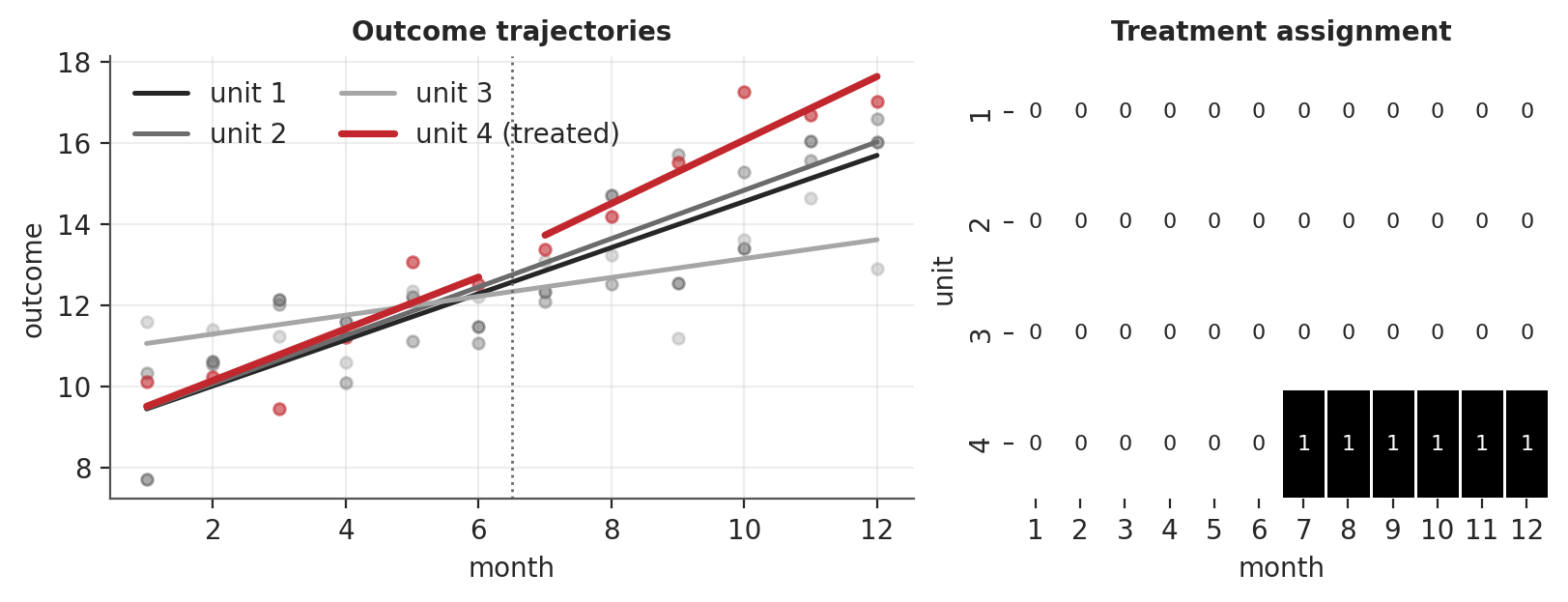
Simulating a small panel, with one unit treated partway through, shows what we are working with.
In Figure 1 we see two views. On the left we see four units’ outcomes over twelve months, with unit 4 (red) treated after month 6 (dotted line) and the controls in grey. Faint points are the raw observations; the bold line-fits abstract each unit into a trajectory, and the treated unit’s fitted level steps up at adoption. On the right we see the identical panel as a treatment matrix, where the outcome values fall away and each cell records only assignment — 0 (light) before treatment, 1 (dark) after.
The matrix sharpens the causal question to the level of a single cell. Extending the potential-outcomes notation of 2 Causal quantities and g-computation from one index to unit and time, let \(Y_{it}(1)\) and \(Y_{it}(0)\) be the outcomes unit \(i\) would realise at time \(t\) with and without treatment. The most granular causal quantity is the cell-level effect.
\[ \tau_{it} = Y_{it}(1) - Y_{it}(0) \]
The fundamental problem now bites cell by cell: in a treated cell we observe \(Y_{it}(1)\) but never \(Y_{it}(0)\), and in an untreated cell the reverse. In the toy panel, unit 4 is treated after month 6, so at month 9 we observe \(Y_{4,9}(1)\) while \(Y_{4,9}(0)\), the counterfactual we need, is missing.
Two sources of leverage
Part II organised its chapters by the threat each one answered; this part inverts that axis. Here the threat is constant. We lack the untreated trajectory from every design, and what varies is how we leverage data to impute the counterfactual trajectory.
The richness of panel data is that it gives us multiple angles on those missing counterfactuals:
- Longitudinal leverage: the treated unit’s own pre-treatment trajectory tells us something about where it would have gone absent treatment.
- Cross-sectional leverage: the untreated units’ post-treatment trajectories tell us something about what common time shocks look like.
Both levers require assumptions about how the treated unit’s untreated trajectory relates to its observed trajectory and to the control units’ trajectories. Every design in this part is distinguished chiefly by which lever it pulls and what it must assume to make that borrowing credible. Part II’s concern with sensitivity and identification carries over, but the panel setting supplies robustness checks of its own. In the panel data setting we can deploy placebo tests to probe the credibility of our estimates by varying treatment dates or panel units.
More observations let us move beyond simple confounding. The Pearlian identification criteria establish a binary verdict. A DAG for \(X \to Y\) is either confounded or not. When we have \(X \leftarrow U_{latent} \to Y\), there is nothing conditioning can offer. The methods in this part can be thought of as attempts to identify and subtract out the confounding effect of \(U_{latent}\). This is a familiar strategy akin to the measurement models in the SEM tradition, but here we use panel data to supply indicator measures of the latent confounder. Placebo tests then probe whether there was sufficient leverage available to plausibly recover \(X \to Y\).
Applying leverage
This part does not aim to survey every named panel estimator.1 Instead, it focuses on a small set of panel designs that represent genuinely different identification situations.
Pre-Post Contrasts: The first chapter of this part, 10 Before and After: Change Scores to ANCOVA, considers the simplest possible panel structure: two time points. With only a before and an after measure, change scores, ANCOVA, and \(2 \times 2\) difference-in-differences all rely on different assumptions about how untreated outcomes would have evolved. Each draws on cross-sectional leverage from a comparison group, longitudinal leverage from the pre-period, or both.
Interrupted Time Series: 11 Interrupted Time Series: No Control Group, Still Causal? then strips out the control group: we’re forced to compare outcomes against expected counterfactuals. There are many observations over time but no contemporaneous control, so the design leans on longitudinal leverage alone, relying on a treated unit’s own pre-intervention history to reconstruct the counterfactual trajectory.
Synthetic control groups: 12 Synthetic Controls and Counterfactual Trajectories confronts the same absence of a ready-made comparison group, but leans on the opposite lever. Rather than asking whether the treated unit’s own history is sufficient, it asks whether a carefully weighted combination of many untreated units’ trajectories can be assembled into a credible synthetic stand-in for the missing counterfactual. The treated unit’s history still matters, but only to choose which untreated units to borrow from. This is a form of cross-sectional leverage.
Difference-in-Differences: From there, the part moves to a different identification regime in 13 Two-Way Fixed Effects: What Repeating Units Reveal: assessing causal interventions across multiple periods and groups, using both levers together. When the panel contains many units observed over many time points, a single \(2\times 2\) contrast no longer suffices. Fixed-effects and event-study methods absorb confounding across time and individuals, allowing credible treatment estimates. But the chapter also shows, by simulation and on real data, how the workhorse two-way model breaks when treatment rolls out to different units at different times, and how cohort-aware event-study models repair it.
Marketing Mix Modelling: 14 Marketing Mix Modelling and Experimental Calibration closes the part with a case where neither source of leverage is enough. A brand’s sales history is a single time series, and the budgets in it chase demand. Spend rises in the weeks planners expect to be busy, so the model has a hard time attributing the credit to the appropriate channel. Delay and decay functions capture how advertising works over time, but historic data no longer separates a channel from the demand that set its budget. The leverage has to be made. A designed lift test changes one channel’s spend independently of demand, and the chapter shows that it helps only when the model can tell designed spend from typical spend.
Taken together, these chapters are meant to give an incomplete survey of a rich ongoing research programme. Once you have surveyed them, you should be able to recognise distinct panel-data regimes, ask which source of leverage they rely on, and judge when a causal question requires more than observational time series alone.
Nor does it cross into epidemiology’s dialect for longitudinal causal inference, where a confounder can be measured repeatedly and itself be shaped by earlier treatment. The focus of the models in this part is on time-invariant confounders, shared time shocks, or a few latent factors combining the two, and none handles that feedback loop between treatment and confounder explicitly. The work of (Robins 1986; Hernan and Robins 2020) supplies a proper accounting of these structures; the g-formula, marginal structural models, and g-estimation were built for exactly that problem, and it is a different identification challenge from the ones worked through here.↩︎