Composing Meaningful Models
A company promotes some of its people and not others, then asks whether promotion made the company better off. The ones promoted are affable and friendly. Managers like people who are good with people, and being good with people is much of what the job rewards. We want to understand the effect of promotions in this setting where the treatment assignment is not randomised. Most consequential interventions are not randomised, but we must reason about their effects anyway.
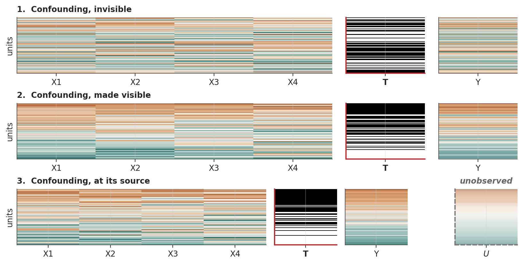
The recipe from the foundations works beautifully when its preconditions are met. The chapters that follow are about what happens when they are not. The figure below shows what that looks like in data, before any model has been fitted. Imagine that friendliness is the unobserved \(U\).
What the Foundations Gave Us
The preceding chapters established a recipe for causal inference. Bayesian modelling gave us a principled approach to uncertainty quantification (1 Bayesian inference: optimisation and sampling). G-computation gave us an algorithmic backbone for causal effect estimation, translating interventional questions into prediction-and-aggregation routines over fitted models (2 Causal quantities and g-computation). DAGs gave us a visual and formal language for encoding our assumptions about data-generating processes (3 Causal thinking with graphs). And the atomic patterns (colliders, chains and forks) showed how to assess rival theories by contrasting DAGs (4 Causal building blocks: forks, chains, and colliders). Throughout, probabilistic programming served as the implementation substrate, translating causal assumptions into generative models we can fit, critique, and refine.
Four lessons emerged from this foundation. First, confounding arises whenever treatment and outcome share common causes, and addressing it requires either conditioning on the right variables or finding designs that render such conditioning unnecessary. Second, the choice of adjustment set is never purely statistical because it demands substantive reasoning about the world. Third, complex causal structures often decompose into simpler subproblems once we identify the relevant conditional independencies. Finally, we also developed a habit of fitting multiple model specifications for each problem. This form of discrete sensitivity analysis stress-tests our conclusions against alternative assumptions.
Threats to Causal Validity
Each chapter in this section confronts a specific way the foundational recipe can fail. Each covers a named threat to causal validity and responds with estimation strategies and model architectures designed to recover credible inference under that threat. The threats escalate in severity, and the models required to address them scale in complexity.
The selection risk threat. You have the right DAG. You know which confounders to condition on. But treated and control units did not arrive at their treatment status by chance. The units selected into treatment, or were selected, in ways that leave some covariate profiles rarely treated, or rarely untreated, so the outcome model must extrapolate where the data are thin. The chapter on propensity scores and information weighting (5 Propensity Scores and Information Weighting) reframes causal inference as a sampling design problem. Just as a surveyor must account for which units were sampled to make valid population inferences, the analyst must account for which units selected into treatment to make valid causal ones.
The unobserved confounding threat. The DAG contains unmeasured common causes of treatment and outcome. No conditioning set among observed variables blocks the backdoor path. This is the harder version of the fork pattern from the foundations. In Figure 1 the confounder \(U\) in \(T \leftarrow U \rightarrow Y\) is latent, and no amount of observable conditioning recovers the uncontaminated causal effect. The chapter on instrumental variable regression (6 Supply, Demand and Instrumental Variables) addresses this by finding exogenous variation that shifts treatment without touching the confounding pathway. The Bayesian framing expresses this as a joint bivariate model of treatment and outcome, where endogeneity appears as residual correlation and the instrument’s validity is encoded directly in the likelihood.
The misspecification threat. The DAG itself may be wrong. With multiple endogenous variables determining one another and latent constructs measured with error, the identification problem shifts from “which variables to condition on” to “have we drawn the right graph at all?” You might object that DAGs are pictures without content: drawing a graph is easy but knowing whether the graph is right is impossible. The chapter on structural equation models (7 Structural Equation Models and Path Diagrams) answers this objection by showing how measurement models, residual covariance patterns, and posterior predictive checks turn graphical assumptions into empirically auditable claims. SEMs give the abstract DAG a concrete diagnostic surface: residuals reveal where the postulated structure strains against the data, model comparison quantifies the cost of alternative specifications, and iterative refinement guided by domain knowledge moves toward defensible causal closure. No single fit-statistic can refute an entire theory of the data generating process. Diagnostics tell you where your graph is failing; only substantive reasoning about the completeness of the graph can tell you whether the causal claims it supports are warranted.
The counterfactual adequacy threat. Models are not merely built to describe history; they are built to project into worlds that do not yet exist. The chapter on discrete choice counterfactuals (8 Discrete Choice Counterfactuals) introduces a counterfactual criterion of adequacy which demands that a model’s structure be rich enough to survive the stress test of hypothetical intervention. Three specific obstacles threaten this criterion: implausible substitution patterns (the simplest models force proportional switching between alternatives, denying market structure), demand endogeneity (observed prices reflect the same demand shocks that drive choices), and preference instability (cross-sectional estimates may not project into counterfactual worlds). Taste heterogeneity is not a nuisance to be controlled but the mechanism by which the model captures individual-level causal structure. When that heterogeneity is validated through out-of-sample prediction on panel data, the model demonstrates that it has captured something real about the decision-making process, establishing stable preference orderings that persist across time and context. We canvass a range of discrete choice models moving from the inadequate multinomial-logit, through the nested-logit to the more robust mixed-logit. All three models answer interventional questions. What improves is whether their substitution patterns survive the counterfactual criterion of adequacy.
The unverifiable assumptions threat. Every preceding chapter rests on an assumption the data cannot fully verify: ignorability for propensity scores, the exclusion restriction for instrumental variables, the completeness of the DAG for structural equation models, the substitution structure for discrete choice. The chapter on sensitivity analysis (9 Sensitivity Analysis: Model Checking and Theory Construction) transforms these binary commitments (the assumption holds or it does not) into continuous perturbations whose consequences can be traced through the posterior. Two modes emerge: model checking, where a well-identified estimate is stressed under escalating violations (a dose-response curve under unmeasured confounding), and theory construction, where sensitivity sweeps discover structural properties of a system (collective judgement under conformity pressure). The chapter closes by mapping this workflow back onto each preceding chapter, identifying the load-bearing assumption in each and showing how to parameterise its violation. This capstone makes explicit what the earlier chapters performed implicitly: the analyst’s task is not to defend assumptions but to measure how much they bear.
Cross-Sectional Data: Mapping the Territory
Across this progression, two themes recur.
The first is the expanding complexity of joint distributions. Propensity scores condition a univariate outcome model on the treatment mechanism. Instrumental variables model treatment and outcome jointly, gaining access to endogeneity through residual correlation. Structural equation models extend to systems of simultaneous equations with latent constructs. Discrete choice models add hierarchical structure over heterogeneous agents. At each step, the joint distribution grows more expressive, the identification problem it addresses grows harder, and the assumptions required to solve it grow stronger. The trade-off is transparent: we gain the ability to recover effects that simpler models cannot identify, but we pay in the strength of what we must defend.
The second is the continuing centrality of DAGs and the importance of structured information flows. In the propensity score chapter, the DAG is simple: we observe the confounders, the treatment, and the outcome, and the main work is compositional. In the instrumental variable chapter, the DAG encodes instrument validity: exclusion and independence. The structural equation chapter shows how the DAG maps the model exactly. The map determines which variables are exogenous, which paths carry direct versus indirect effects, and whether identification is achieved at all. In discrete choice, DAG reasoning diagnoses endogeneity and guides control function design. The foundations introduced DAGs as a visual convenience for simple systems; these chapters show they are load-bearing architecture for complex ones. The DAG remains the map; the joint distribution is the territory and testing ground.